主に大学入試を過学習してしまったがために学部の計算がすらすらできなくなってしまった方(※) に向けたまとめノート。
(※) を見て吐き気を催す方等。私とか私とか、私とか。
双曲線関数とその逆関数、およびそれらの微分, 積分について主に扱います。
Wikipedia の当該記事を見れば全部書いてあるんだろうけど、普段の計算に支障が出ないよう普段から頭に入れておくべきだと思われる公式を 1 つのページに収めておくことはそれなりの価値があると思うので、とりあえずこのかたちで置いておくことにします。
なお、本記事に載せてある図を作成するための TikZ のコードは、lualatex による動作を確認しています。platex を使用している方は \documentclass のオプションに dvipdfmx 等を追記したのちタイプセットしてください*1。
双曲線関数
定義
| |
|
|
|
| 定義域 | |
|
|
| 値域 | |
|
|

TikZ コード
% hyp.tex
% author: bakkyalo
\documentclass{standalone}
\usepackage{tikz}

\begin{document}
\begin{tikzpicture}

% origin
\draw (0, 0) node[below right] {O};

% axes
\draw[-stealth] (-4, 0) -- (4, 0) node[right] {$x$};
\draw[-stealth] (0, -4) -- (0, 4) node[above] {$y$};

% y = 1
\draw[dashed] (-3.5, 1) -- (3.5, 1);
\draw (0, 1) node[below left] {$1$};

% y = -1
\draw[dashed] (-3.5, -1) -- (3.5, -1);
\draw (0, -1) node[below left] {$-1$};

% graph
\draw[blue, thick, domain=-2.0:2.0] plot (\x, {sinh(\x)}) node[right] {$\sinh x$};
\draw[red, thick, domain=-2.0:2.0] plot (\x, {cosh(\x)}) node[left, red] {$\cosh x$};
\draw[green, thick, domain=-3.0:3.0] plot (\x, {tanh(\x)}) node[below, green, fill=white] {$\tanh x$};

\end{tikzpicture}
\end{document}
相互関係
- とりあえず大事なのは2つ目。
が直角双曲線
の媒介変数表示になっていることが分かる。
- 実用の観点から
の形でも把握しておく。- 3, 4 つ目は応用的な積分計算等に使うかもしれない。 (あまり見たことないけど)
加法定理
2倍角の公式
半角公式
微分公式
積分公式
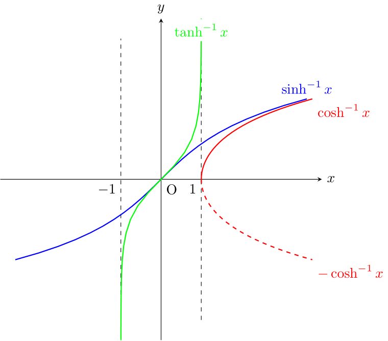
逆双曲線関数
のみ単射でないため、上半分と下半分に分かれる。
| |
|
|
|
| 定義域 | |
|
|
| 値域 | |
|
|
TikZ コード
% ahyp.tex
% author: bakkyalo
\documentclass{standalone}
\usepackage{tikz}

\begin{document}
\begin{tikzpicture}

% origin
\draw (0, 0) node[below right] {O};

% axes
\draw[-stealth] (-4, 0) -- (4, 0) node[right] {$x$};
\draw[-stealth] (0, -4) -- (0, 4) node[above] {$y$};

% x = 1
\draw[dashed] (1, -3.5) -- (1, 3.5);
\draw (1, 0) node[below left] {$1$};

% x = -1
\draw[dashed] (-1, -3.5) -- (-1, 3.5);
\draw (-1, 0) node[below left] {$-1$};

% graph
\draw[blue, thick, domain=-2.0:2.0] plot ({sinh(\x)}, {\x}) node[above] {$\sinh^{-1} x$};
\draw[red, thick, domain=0:2.0] plot ({cosh(\x)}, {\x}) node[below right, red] {$\cosh^{-1} x$};
\draw[red, thick, dashed, domain=0:-2.0] plot ({cosh(\x)}, {\x}) node[below right, red] {$- \cosh^{-1} x$};
\draw[green, thick, domain=-4.0:4.0] plot ({tanh(\x)}, {\x}) node[below, green, fill=white] {$\tanh^{-1} x$};

\end{tikzpicture}

\end{document}
log による表現
を
について解くと
となり、上半分を
、下半分を
として採用する。両者が両立することは簡単な
の計算によっても確かめられる。
微分公式
練習問題 — 懸垂線
紐の両端を固定させて垂らした時にできる曲線は懸垂線と呼ばれます。
この方程式が で書けることを (少々ガバいですが) 確認してみます*2。
問題設定

TikZ コード
% cat.tex
% author: bakkyalo
\documentclass{standalone}
\usepackage{tikz}
\usetikzlibrary{angles, quotes}

\begin{document}
\begin{tikzpicture}[scale=0.9]

% coordinates
\coordinate (O) at (0, 0);
\coordinate (M) at (1, {cosh(1) - 1});
\coordinate (P) at (2, {cosh(2) - 1});
\coordinate (dP) at (2.4, {sinh(2)*2.4 + cosh(2) - 1 - 2 * sinh(2)});
\coordinate (H) at (2.5, {cosh(2) - 1});

% points
\fill (O) circle[radius=1mm] node[below left] {O};
\fill (P) circle[radius=1mm] node[left] {P};

% axes
\draw[-stealth] (-4, 0) -- (4, 0) node[right] {$x$};
\draw[-stealth] (0, -1) -- (0, 5) node[above] {$y$};

% graph
\draw[thin, domain=-2.4:2.4] plot (\x, {cosh(\x) - 1}) node[above] {$y = f(x)$};

\draw[ultra thick, domain=0:2.0] plot (\x, {cosh(\x) - 1});

% gravity
\draw[-latex, red, thick] (M) -- (1, -1) node[midway, right] {$\lambda l g$};

% tension
\draw[-latex, blue, thick] (O) -- (-1, 0) node[below] {$T(0)$};
\draw[-latex, blue, thick] (P) -- (dP) node[right] {$T(x)$};

% angle
\draw[thin] (P) -- (H);
\draw pic[-latex, "$\theta$", draw=black, angle eccentricity=2, angle radius=3mm] {angle=H--P--dP};

\end{tikzpicture}
\end{document}
求める曲線を とおき、図のように紐の極小点を原点とする
座標をとって、点
における接線と
軸とのなす角を
とおきます。すると、
です。
紐の質量線密度を 、重力加速度を
とし、点
における張力の大きさを
とおいたとき、
に加わる力のつりあいの式を考えます。
*1:ただ、自分の環境ではなぜか白紙の 2 ページ目が生成されてしまいます。
*2:2年生でやる解析力学では変分法の練習問題として与えられることが多いと思いますが、紐のつりあいの式から微分方程式を作って解くことができるので、この方法で行くことにします
*3:材料力学 (と多少の曲線曲面論) の力を借りると、 の一階微分はたわみ角 (
軸方向と接線方向のなす角) を表していることが分かります。つまり、
というのは「
におけるたわみ角は
です」と言っている訳で、天下り的になりますがそうなるように問題を設定したという事になります。
における張力がちょうど
方向になっているのがそれによって現れていますね。なお、今回は関係ないですが、
の二階微分は曲げモーメント、三階微分は剪断力を表しており、高階の微分方程式の境界条件を与えるのに重要になってきます。この辺の話もいつか記事にまとめたいとは思っていますが、いつになるんでしょうね。。。